6.1 INTRODUCTION
The main feature of our instrument is the implementation, for the first time in the filed of electrical measurement, of an FFT algorithm, which minimizes the phase error due to the
short-range leakage. Moreover, as we already seen from the previous chapters, the measure is performed in real time.
The algorithm is based on a paper published by Ferrero and Ottoboni [1].
Before going into the details, in the next section we briefly describe the considerations that lead us to the use of this algorithm.
6.2 FFT OF A PERIODIC SIGNAL
A sequence of sampled data may be symmetrical or not, with respect of the time origin.
Let us consider first the case of symmetric sequence.
Let s(t) representing a periodic signal with period Ts and S(f) its Fourier1 transform.
Suppose also that the sampling frequency fc=1/Tc, has the right value to match the Nyquist requirements.
If we take 2N+1 samples, evenly spread over the range [-NTc, NTc], the resulting sequence {s(k)}
is symmetrical with respect to the sample s(0), where the index k=0 represents the time origin.
Now, if we consider an asynchronous sampling
6.1
the sampling of the signal s(t) mathematically is equivalent to the following product
6.2
where g(t) is a train of Dirac impulses time limited.
6.3
The Fourier transform of g(t) is:
6.4
The above equation also represents the Fourier transform of a rectangular window Tc(2N+1) points long.
From the convolution theorem, the Fourier transform of p(t) is given by
6.5
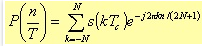
P(f) can be obtained from the sampled values of s(t) by
6.6
or, in case of evaluation through digital techniques, by
6.7 a
Now, because of the asynchronous sampling, we can observe two main effects:
1. G(f) has zeros for frequency values that differ from the harmonic frequencies of s(t).
This means that when we calculate the n-th harmonic component using the above equation, all the harmonic components give their own contribute rather than the n-th
component alone.
This phenomenon of harmonic interference depends on both S(f) and G(f), and it is the responsible for the so-called long-range leakage,
which affects both the phase and the amplitude.
One way to reduce this interference between the harmonic components, that is the long-range leakage error, is by the use of specific windows.
Examples of these windows have been already described in the chapter about the FIR filtering.
Indeed these windows exhibit lower ripple attenuation over the side lobes (see figures from 4.2 to 4.7.)
2. The main lobe of G(f) reaches the maximum value for frequencies equal to n/T, where n is an integer in the range [-N, N].
These frequencies differ from the harmonic frequencies of the signal s(t); it follows an error that affects only the harmonic amplitudes.
This error is called short-range leakage error; in order to reduce this kind of error, you could use specific windows known as FLAT TOP windows
(see figures 6.4, 6.5, and 6.6).
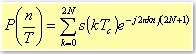
In the more generic case of a sampled data sequence no more symmetrical with respect to the time origin, the algorithm representing the FFT is
6.7 b
Now, for a generic asymmetric sequence, n varies from 0 to 2N.
This results in a Fourier transform of the time limited impulse train, which has the following form
6.8
1
We mean transform in the field of Distribution theory.
6.3 THE IMPLEMENTED ALGORITHM
In the previous chapter, we saw that the use of the Radix 2 FFT requires sequences with a number of data, which is a power of two.
Generally, these sequences are not symmetrical with respect to any of their terms: this means to have the errors previously described, and in particular,
the phase error coming from the short-range leakage, which is the dominant error.
Fortunately, a symmetrical sequence can be obtained starting from an asymmetric one, in the following way.
Let us consider a signal s(t) sampled according to the Nyquist condition; the resulting sequence is generally not symmetric.
6.9
Once defined, however, the time origin
6.10
it is possible to consider the new sequence
6.11
such that
6.12
We suppose that the terms of this sequence are the samples of s(t-t0) in t0=(N-1/2)Tc within the range
[-N, N-1], so now the sequence is symmetrical with respect of the point t0.
The Fourier transform of the sequence
6.13
is given by the following expression
6.14
i.e.
6.15
If we set i=-(h+1) in the first summation, it follows that
6.16
The two summations are not ready to be evaluated directly as FFT terms because of the exponential terms e±jπni/N instead of the terms e±j2πni/N.
The solution is to add N null points to each sum in the range N ≤ h,i ≤ 2N-1. Obviously, the result does not change.
6.17
At this point, we have to calculate two FFT on 2N point each, with half of the points that are null data.
About the input order of the signal points, using the FFT algorithm with time decimation the bit reversing is performed only on the n not null data.
In fact, it is enough to alternatively place the zeros between an original point and the next one.
In this way, it is also possible to considerably reduce the first computational stage of the FFT:
in fact, as you can see from the figure 6.1, if x(j)=0, the two outputs will have the same value as the input value x(i), which is not null a priori.
Fig. 6.1.
Therefore, instead of adding a signal of N null data, we preferred to double each input data in order to obtain an input signal as x(0), x(0), ..., x(i), x(i), ....
In this way, we avoid the first computational stage of the FFT saving time (figure 6.2b).
The second computational stage can be avoided too (figure 6.2c.)
In fact, note that in the first memory location you store the sum between the first point and the third one, while in the third memory location you store their difference.
In the second memory location there is the original point, and in the fourth one, there is the third point with opposite sign.
Fig. 6.2. The first three stages of the implemented FFT algorithm.
a): Buffer of the generic data X with the N added zeros.
We do not need a bit reversing because it is enough that the zeros come between the original data samples.
b): Theoretic configuration of the input data at the first FFT stage, and c) at the second stage with the final results.
In this way, it is possible to reduce the first two FFT stages into one only stage, and to start the calculation of the FFT from the third stage.
Moreover, the fact that the original signal has positive weight factors instead of negative, as for the conventional FFT, means that is like to perform the FFT on a signal,
which is out of phase for 180°.
In fact, applying the algebraic properties in the complex domain to the first summation, we have
6.18
By replacing the above expression in the original one, we obtain
6.19
The terms inside the brackets represent two real FFT performed as there were two different signals.
Figure 6.3 briefly shows the main flow diagram of the algorithm where the two summations are calculated as two FFT;
the second step labeled as Data ordering, regards the harmonics ordering to reconstruct the spectrum of the original signal.
The results from the first brackets are conjugated.
Then, each data is weighted by an exponential factor.
Finally, the result is the sum of the two data.
Fig. 6.3. General Flow Diagram for the FFT algorithm with phase error correction.
We obtain in this way the harmonics of the original signal, minimising the phase error.
6.3 THE IMPLEMENTED WINDOWS
Generally, the use of a FFT can leads to wrong results in presence of phenomena such as the aliasing or the spectrum leakage.
The former effect can be prevented by a proper use of the Shannon's sampling theorem, and a lowpass filter for the input signal.
About the latter effect, the FFT looks at the signal to be analysed as if it were a periodic signal with period equal to the observation window of time.
If this range of time is exactly an integer multiple of the signal period, the spectrum leakage effect does not take place.
On the contrary, there are discontinuity points at the border of the observation range with a consequent degradation of the spectral lines [1].
As for the FIR filters, for the FFT the use of proper windows can considerably reduce discontinuity at the border of the observation range,
attenuating the error due to the harmonic interferences.
This is the reason why we implemented with the FFT, almost the same windows (Rectangular, Hamming, Hann, Blackman, Blackman-Harris, and sin6)
most of them have been already described for the FIR filters.
Moreover, we add also Flat Top type windows with 3, 4, and 5 coefficients. Their name comes from the fact that the main lobe is generally flat at the top
(see figures 6.4, 6.5, and 6.6.)
A typical use of these windows is to reduce the short-range leakage errors.
Fig. 6.4. Flat Top with 3 coefficients.
Fig. 6.5. Flat Top with 4 coefficients.
Fig. 6.6. Flat Top with 5 coefficients.
The generic equation is
6.20
where Δfn is the frequency resolution, Δt is the time interval between two samples, and M is the significant number of spectral lines of the window.
Asserting some conditions such as the coefficients normalisation
6.21
and those that regulate the asymptotic behaviour of the window
6.22
you can obtain windows with three, four, or five coefficients. In particular
Table 6.1.
6.3 LABVIEW ALGORITHMS
We implemented two sub-systems for the spectral analysis: one for the conventional FFT and one for the FFT with the phase correction algorithm.
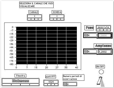
Figures 6.7 and 6.8 show the control panel of the conventional FFT.
The Front panel of the FFT with the phase correction algorithm is almost the same with very little differences.
In the conventional FFT case, it is possible to select up to 8 channels for a maximum of 1024 points per channel.
In the case of the FFT with the phase correction algorithm, it is possible to select up to 4 channels always with a maximum of 1024 points per channel.
This comes from the fact that the latter FFT case requires double the space of memory with respect to the conventional one.
This is the only difference concerning the control panels for the two FFT cases.
Both panels provide a trigger control, analogical or digital, with the ability to select the source channel for the trigger.
The sampling frequency clock can be external or internal.
If the user selects the internal clock, once selected the desired frequency value, a display shows the actual frequency allowed by the acquisition boards.
Through another input control, it is possible to select the number of points on which to perform the FFT: it can be 64, 128, 256, 512, or 1024.
In the same control panel figures, it is possible to see a window selector, and two displays that show the instantaneous value of the module and the phase of the selected spectral lines.
The module is in volt while the phase in degree.
A switch with a led is used to start and stop the instrument.
During the measurement, the spectrum is displayed.
The spectrum display provides two input controls to select for which signal you want the spectrum displayed in that moment.
Fig. 6.7. Partial view of the control panel for the FFT.
Fig. 6.8. The other part of the control panel for the FFT.
Regarding the graphical programming language to handle the front panel (see figures 6.9 and 6.10),
there are two main sequences: the first one manages the acquisition boards through a Code Interface Node (CIN), which is programmed in C.
It configures the acquisition boards accessing the status registers, depending on the input parameters selected from the control panel.
The C code resides inside the CINRun that, as already described in the chapter 2, is invoked only when the user switch on the instrument from the control panel.
Fig. 6.9. First sequence of the block diagram for the conventional FFT. This sequence handles the acquisition boards set up.
Fig. 6.10 a). First half of the second sequence of the block diagram for the conventional FFT.
Fig. 6.10 b). Second half of the second sequence of the block diagram for the conventional FFT.
It is worth pointing out that the second sequence has two CINs: the first one (see figure 6.10 a) regards the DSP.
Its tasks are to download the software into the DSP and to run it as soon as the LabVIEW itself is executed.
This CIN is in charge to pass to the DSP the communication variables, the control panel parameters, and the trigonometric tables necessary to perform the FFT;
moreover, the CIN displays the data that the DSP updates after each processing.
During the turning off phase of the virtual instrument, the CIN set the DSP in an IDLE state, so that LabVIEW will be able to upload the DSP with a new program.
In order to perform all the above described tasks from one CIN only, we differentiated the code into different CIN parts:
the CINInit, which is invoked as LabVIEW load the instrument, first loads the code on the DSP;
then, allocates all the necessary memory locations to store the variables the DSP needs to "see".
These variables are defined outside the CINInit because shared by the CINRun and the CINDispose also.
These variables are set to the default values, which are displayed on the front panel at the time in which the instrument panel is opened.
The variables are passed to the DSP by reference rather then by value, because once started the DSP, the DSP becomes the master of the communication with the hosting Macintosh.
For each address to be passed to the DSP, there is a memory alignment check.
In fact, the memory alignment for the DSP is of 32 bits (one word), and a communication is possible only if the unit connected to it has the same memory alignment.
In case of error detection, the code execution is halted and the DSP will not be started. This is the reason why each parameter of integer type, needed by the DSP, has been defined
as of 32-bit type (long). Similarly, for each parameter of floating point type we used a 32 bits floating point representation.
Once the code and the addresses are loaded on the DSP, the DSP start its execution.
The CINDispose is called both at the time of the instrument loading phase, and at the time of the instrument closing phase.
In this part of the CIN, there is a flag that the DSP should read before each processing, in order to know whether to keep going with the processing or not.
If not, the DSP restore the initial conditions and goes into an IDLE state, ready to be used again, maybe with a new application.
The way this flag is used is the following one: when the flag is set, the DSP knows it has to stop.
The CINDispose always set this flag. Then the CINInit, when called, clear the flag before running the DSP.
When the virtual instrument is closed, LabVIEW invokes again the CINDispose that set again the flag.
Note that after setting the flag, the CINDispose executes a short waiting loop, to let the DSP to complete the processing, and to read the flag on the host.
The CINRun does not start automatically, but only when the virtual instrument is switched on.
The job performed by the code inside this part of the CIN regards three different issues: first, it has to keep updated the CIN output from the DSP results,
so that LabVIEW can display the data. Second, it has to check continuously if any of the control parameters placed on the front panel has been changed by the user
(like for instance, a change in the number of points on which perform the FFT, a change in the number of channels, or a new window selection, and so on.).
In this case, the lookup tables concerning the windows and the trigonometric weights for the FFT butterflies are calculated again; a secondary flag is set to notify the
DSP that a parameter change occurred. The DSP stop its execution, load the new lookup tables and the new parameters, clear the flag in LabVIEW, and restore its processing execution.
The second CIN in figure 6.10 b, checks, and eventually changes, the signs of the harmonic components and their relative real and imaginary parts. In fact the Sorensen algorithm, even if provides the correct information necessary to calculate the harmonic modules, introduces a systematic error, hence easily correctable, about the harmonic phases. In practice, Sorensen sets each harmonic out of phase for an amount equal to 90° multiplied by the harmonic order. Therefore, this second CIN corrects this phase error bringing back the complex vectors, which represent the harmonics, to their proper quadrant.
For the calculation of the instant value of the module and the phase of the harmonic components, we used the icons provided by LabVIEW (figure 6.10 b.)
6.6 DSP ALGORITHMS
If not otherwise declared, the following description holds for both the conventional FFT and the FFT with phase error correction algorithms.
The software executable code comes from assembling and linking the objects of four distinct programs:
the main program (Main), an interrupt service routine, an FFT routine, and a procedure to translate the floating point values, which use standard IEEE representation in host environment,
to the Texas Instrument (TI) representation, used by the DSP, and vice versa.
All this code has been written in assembly language.
The resulting executable code has been placed on the ONCHIP memory.
All the pointers to the different memory locations have been placed in the same memory space where the executable code is, in order to reduce a continuous paging.
On the other hand, the variables with the LabVIEW addresses have been placed in the Dual Access memory because this is the only area the host can access directly without using interrupts.
In fact, the use of interrupts, in this specific case, will result in a more complex code with a degradation of the execution time performance.
Always in Dual Access memory, we allocated space for the lookup tables, which values are calculated in LabVIEW, and the data to be processed.
This lets us, upon format conversion, a direct data transfer from the DSP to the hosting Macintosh.
The Main program performs the following tasks:
1. It disables the interrupts number 1 and 2 respectively for the RTSI bus and the DMA.
2. It loads the control parameters from LabVIEW, which already passed to the DSP their addresses in the host.
Then reads on how many points and channels it has to perform the FFT, and stores these values in the Dual Access memory.
3. After initialising the pointers to the different buffers, whose number depends on the number of channels used, it loads the lookup tables of the selected window from LabVIEW.
It makes the floating-point conversion from the IEEE representation to the TI one. It loads and converts the lookup table for the FFT butterflies.
The FFT with phase error correction requires a further lookup table with the exponential weights for the harmonics (see previous sections.)
This step does not exist for the conventional FFT.
1. It initialises the variables that represent the argument to be passed to the FFT routine.
At this point, the phase of reading LabVIEW parameters is completed, and the Main clears the flag about the "change of parameters" on the host.
2. It loads the interrupt vector 1.
3. It configures the DSP Control Register and clears all the data memory buffers.
4. It configures the internal timer and the addresses where to write into the acquisition boards.
It loads the address of the Soft A/D Clear Strobe Register of the acquisition boards, in order to clear their FIFO memories.
5. It enables the interrupt 1 for the acquisition data ready, because in this time the sampling is already started. From here, the real time processing also starts.
6. The Main starts the wait loop where the processing resides along with the data transfer to the hosting Macintosh: first,
the Main is in an IDLE state waiting for the interrupts.
For each interrupt, the Main leave its idle state and check, first of all, whether or not the LabVIEW set the "end-of job" and/or the "change of parameters" flags.
In the former case, it halts the execution and jumps to the end of the program. In the latter case it jumps to the beginning of the program (step 1.)
7. It then checks the number of received interrupts in order to understand if there are enough data to start the processing.
In fact, in case of four channels, for instance, for each acquisition interrupt, there are 512 points per board (256 per channel) in the DSP Dual Ported memory.
To be able to perform a 1024 points FFT, it needs to wait for 4 interrupts.
8. Once there are enough data, it starts the nested loops of the FFT1 per channel.
Before calling the FFT routine, the data are weighted with values taken from the lookup table of the selected window.
Only for the algorithm one with phase error correction, there is a further step about the data ordering and harmonics weighting with the values coming from the exponentials lookup table
(see figure 6.3.)
1. A processing stage is completed. The Main change the floating point representation of the data to the IEEE format, consistent with the Macintosh environment, and then send the data to the host memory, so that can be displayed. The code jumps back to the step 9 to wait for new interrupts.
2. The last step.
The Program Counter is here only if LabVIEW set the "end-of-job" flag.
Before entering in the IDLE state, the DSP enables the interrupt letting the host to download a new application.
It is at this time that the DSP is not the Master anymore, and waits for new instructions.
Concerning the interrupt service routine, its tasks are the following
1. It saves all the DSP registers on the stack.
2. It configures the DMA Controller for the data block transfer mode from the acquisition boards to the DSP Dual Ported memory.
The input samples are packed so that for each transferred word there are two one-word samples.
3. It checks if the transfer is completed by polling.
4. Once the data transfer via DMA from the first acquisition board is completed, it prepares the data transfer from the second acquisition board.
5. The DSP starts to unpack the data sent by the first acquisition board and places the unpacked data into the Dual Access memory. In the meanwhile, the new data are coming from the second acquisition board via DMA over the NuBus.
6. It checks if the transfer from the second acquisition board is completed by polling.
7. The DSP starts to unpack the data sent by the second acquisition board and places the unpacked data into the Dual Access memory.
8. It restores the DSP registers from the stack and returns to the Main program.
The data unpacking and transferring is different depending on the number of channels in use. In fact, the algorithm has to understand from which of the channels the unpacked data come from, and has to place it in the proper Dual Access memory location consequently.
For the floating-point format conversion routines, we used and corrected, the routines quoted by the National Instruments manuals.
1 One FFT for the conventional case and two FFTs for the one with phase error correction.
6.7 EXPERIMENTAL RESULTS
In this section, we report the experimental results regarding the maximum frequencies that allow a real time processing.
Conventional FFT on 1024 points.
Table 6.2.
FFT with phase error correction on 1024 points.
Table 6.3.
The polling information is referred to the time needed by the DSP to check if there are enough input samples to be processed.
This time interval is necessary to guarantee that no overflow will occur in the acquisition boards.
In fact, we could set other time values, but we had data overflow on the acquisition boards.
These values come after a time estimation we did on the processing time required by the DSP.
Then, these time intervals have been verified run time.
Indeed, the optimal time interval depends on both the number of channels used, and on the points number.
For both the tables, in the first row there is the polling time optimised for the use of two channels.
The second row is the polling time optimized for 4 channels. The third row for the 8 channels (only for the conventional FFT).
In our design, we preferred to optimise the configuration where there are two channels only, and 1024 points.
About the other configurations left, we observed lower values of the maximum sampling frequencies, with differences from zero to some kHz, than the selected configuration case.
In fact, the maximum sampling frequencies distribution as a function of the polling time intervals shows a flat local maximum for intervals less than the evaluated one and it
decreases quicker for greater intervals than the our selected polling time. A similar behaviour has been already seen for the filters.
For instance, in the case of a polling interval equal to 3916ns (conventional FFT) the maximum frequencies are:
89685Hz 45871Hz 24008Hz
for 2, 4, and 8 channels respectively.
Finally, it follows a comparison between the two FFT implementations.
Generally, the phase error for the FFT with the phase error correction is of the order of 10-3 radians vs. 10-2 radians of the conventional FFT.
As for example, we consider an input periodic signal with the fundamental harmonic at 50Hz, given by the following expression.
6.23
Let us consider an asynchronous sampling (i.e. a sampling frequency slightly different from 12800Hz), both the FFTs on 1024 points, and a Blackman window.
Moreover, the input signal is triggered on the rising edge after the zero crossing.
We can measure the following phase error on the fundamental harmonic:
2° 57' Absolute phase error for the conventional FFT, and calculated with respect to the time origin t0.
0° 15' Absolute phase error for the new FFT, and calculated with respect to the time t0=(N-1/2)Tc,
where N is the number of the samples and Tc the sampling period [1].